By David M.
Randomly Assign Names to groups
We cover how to randomly assign names to groups in excel. In other words, we will assign each of the 30 people in this table here to a group, based on the group size that we select.
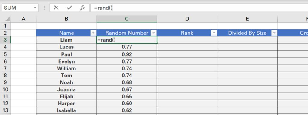
To start, we’ll use the RAND function to assign Liam a random value between 0 and 1. We can double click the bottom right hand corner to bring this formula down for all subsequent names.

However, you’ll notice that when we change the value of other cells, the RAND function re-calculates. To prevent this, we can copy all of the random values, right click our selection, click paste special and then select values.
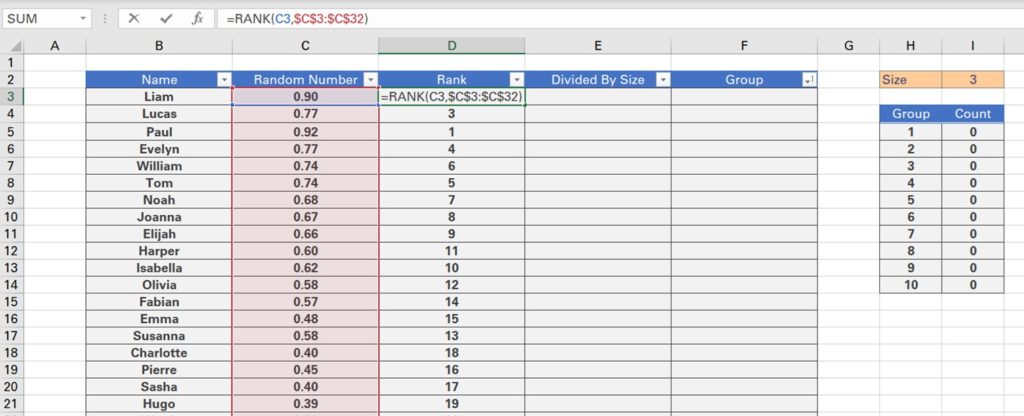
Next, we will use the RANK function to rank each random number from largest to smallest. Here we first input the random number, followed by the range. We will also add absolute references by clicking the F4 key to ensure the table array we selected remains static when we bring the formula down.

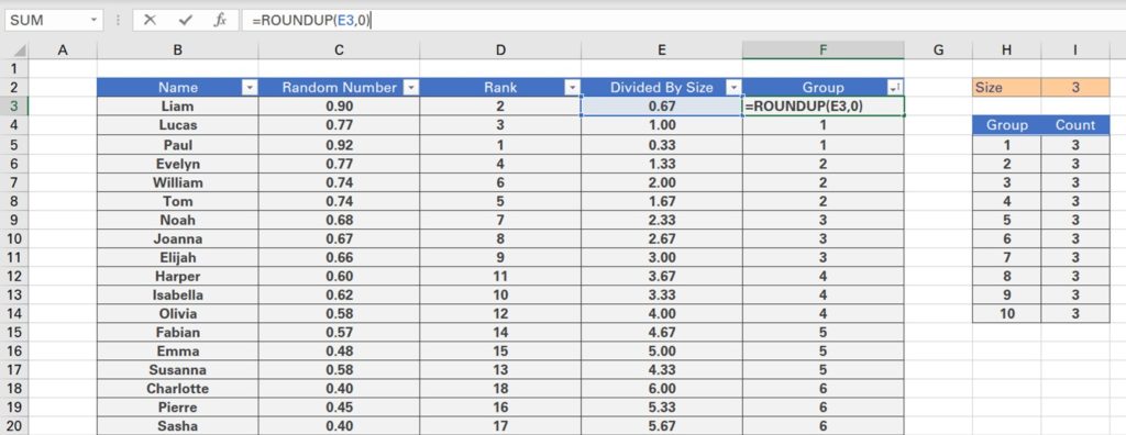
We can then divide each person’s ranking by the size of the group, in this case 3, again adding absolute references. This allows us to determine in which group each person should be.
However, since this column contains decimals, we can round each figure up using the ROUNDUP function. We can then filter this column by clicking Alt + A + T and selecting smallest to largest to get a better idea of the group representations.

Finally, we can test how many people are in each group by using the COUNTIF function. We first input the group column, using absolute references followed by the group we are searching for.
There are 3 people in each group and therefore we’re meeting our size criteria. Let’s test a different group size, such as 8. Since, we have 30 names, the first 3 groups will have a group size of 8 while the last one will have the remainder of people, which is 6.