
By David M.
Dynamic Charts That Update Automatically
Dynamic charts are useful when we want a chart to adjust automatically based on changes in the size of a table array.
To start, let’s insert a static chart. To do this, we will select the table array. We will then enter the insert tab and select the scatter chart icon and click more scatter charts. This chart nicely shows the sales over time. However, when we add additional data, the chart does not adjust to display this as it is static and not dynamic.
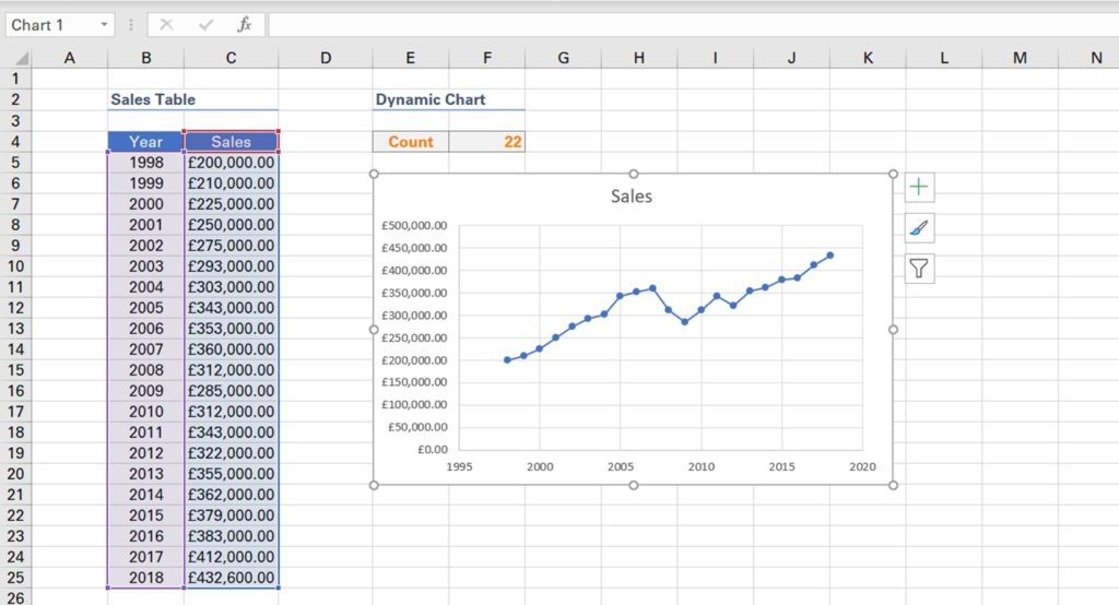
To overcome this, we need to add dynamic ranges. Firstly, we can use the COUNTA function to count how many cells are populated in our table array. This will later help us make our range dynamic as the value in this cell will adjust when we change the size of the table array.
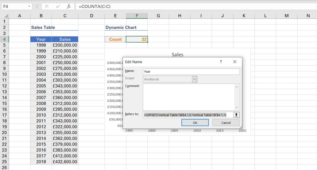
We can then define the named range by entering the formulas tab and clicking define name. Let’s call our first dynamic range Year as it will refer to the year column. Here we enter =OFFSET, we first input the reference cell which is B4, we then type 1, as we want to go 1 row down from this reference cell, we then enter 0 as we’re only concerned with the year column. Next, we can consider the height of the range, given by the cell F4 which we calculated earlier minus 1 as we do not want to include the year heading which is currently included within the COUNTA calculation. We can then type 1 as our range is 1 column wide.
We can enter the name manager, copy the formula we just wrote for the Year range and apply it to the Sales range. The only change we will make is change the reference cell from B4 to C4 so that it refers to the Sales heading.
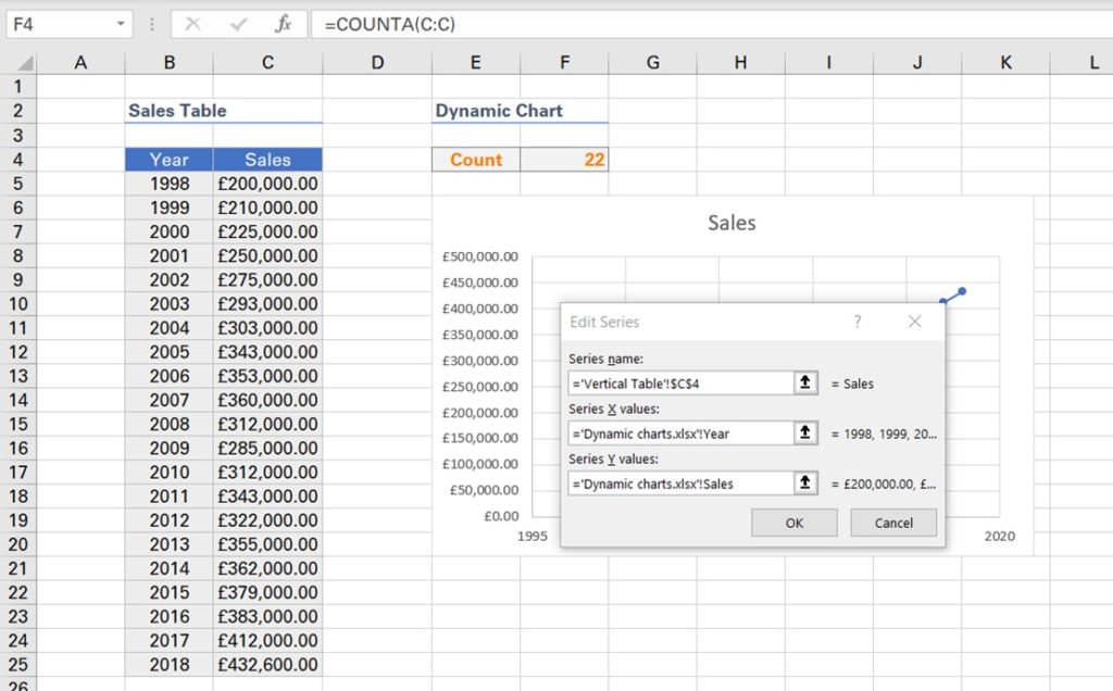
Now that the dynamic ranges are ready, we can right click our chart and click select data. We can then click edit and for series X we will replace the static range for the dynamic year range. For series Y we can apply the dynamic sales range.
When we add an extra data point to the table array, the chart now adjusts to reflect the newly extended range.